Basic information needed to develop models will apear here.
Every model in TCLB is defined by a subdirectory of models.
The conf.mk file stores some additional settings for a model, but it also tells TCLB that this directory is in fact a model.
General information
Each model consit 2 most important files: Dynamics.c and Dynamics.R, what goes where(logic, settings, quantities)
conf.mk
ADJOINT = 1
This file contains information needed during compilation. It allows compilation of diferent versions of a model(from the same Dynamics.c and Dynamics.R). To do so you need to set OPT variable in conf.mk first. E.g:
OPT="(A+B)*C"
This will add three optional functionalities: A,B, and C - called Options. The summation means that two options are exclusive (you can have A or B), and multiplication allows for their combination (you can have A, C and both). The mechanism allows to compile a model for all the resulting combinations. The name of the model is created by adding the option after an underscore. In this case:
| Model | A | B | C |
|---|---|---|---|
| model | |||
| model_A | x | ||
| model_B | x | ||
| model_C | x | ||
| model_A_C | x | x | |
| model_B_C | x | x |
All these models are compiled from the same Dynamics.R and Dynamics.c, but with different options set to TRUE or FALSE in the Options R variable. One can switch on and off parts of the code with:
if (Options$A) {
# code for option A
} else {
# code without option A
}
or in pure C/C++, with:
#ifdef OPTIONS_A
// code for option A
#else
// code without option A
#endif
Dynamics.R
In this file all
- AddField - Variables (for instance flow-variables, displacements, etc) that are stored in all mesh nodes.
Dynamics.ccan access these fields with an offset (e.g. field_name(-1,0)). If the access pattern is repeating you can define a density that predefines a specific offset. Such densities are gathered, and the resulting memory access is optimized.
AddField( name="Name", dx=c(-1,0), dy=c(0,0), dz=c(-1,1), comment='Some comment')
If there is -1,1 access pattern you can use a shortcut:
AddField(name="u", dx=c(-1,1), dy=c(-1,1))
# same as
AddField(name="u", stencil2d=1)
- AddDensity - Variables loaded from
Fieldswith a predefined offset:
AddDensity( name="Name", dx=1, dy=0, dz=0, comment='Some comment')
It is possible to automate the process and add Density for each possible direction(here for d3q27 model):
x = c(0,1,-1);
P = expand.grid(x=0:2,y=0:2,z=0:2)
U = expand.grid(x,x,x)
AddDensity(
        name = paste("f",P$x,P$y,P$z,sep=""),
        dx   = U[,1],
        dy   = U[,2],
        dz   = U[,3],
        comment=paste("density F",1:27-1),
        group="f"
)
As a result, the densities will have the following offset:
$ R

> x = c(0,1,-1);
> P = expand.grid(x=0:2,y=0:2,z=0:2)
> U = expand.grid(x,x,x)
> x
[1]  0  1 -1
> P
   x y z
1  0 0 0
2  1 0 0
3  2 0 0
4  0 1 0
5  1 1 0
6  2 1 0
7  0 2 0
8  1 2 0
9  2 2 0
10 0 0 1
11 1 0 1
12 2 0 1
13 0 1 1
14 1 1 1
15 2 1 1
16 0 2 1
17 1 2 1
18 2 2 1
19 0 0 2
20 1 0 2
21 2 0 2
22 0 1 2
23 1 1 2
24 2 1 2
25 0 2 2
26 1 2 2
27 2 2 2
> U
   Var1 Var2 Var3
1     0    0    0
2     1    0    0
3    -1    0    0
4     0    1    0
5     1    1    0
6    -1    1    0
7     0   -1    0
8     1   -1    0
9    -1   -1    0
10    0    0    1
11    1    0    1
12   -1    0    1
13    0    1    1
14    1    1    1
15   -1    1    1
16    0   -1    1
17    1   -1    1
18   -1   -1    1
19    0    0   -1
20    1    0   -1
21   -1    0   -1
22    0    1   -1
23    1    1   -1
24   -1    1   -1
25    0   -1   -1
26    1   -1   -1
27   -1   -1   -1
>
Observe that:
f_100 == f_100(-1,0,0) # the value is read from the left (`x=-1` direction) <==> it is streamed to the right (`x=1` direction).
and
f_200 == f_200(1,0,0) # the value is read from the right (`x=1` direction) <==> it is streamed to the left (`x=2` direction which is a convention to store the `-1` in the name of the variable).
Have a look at the picture below - it presents the memory layout.
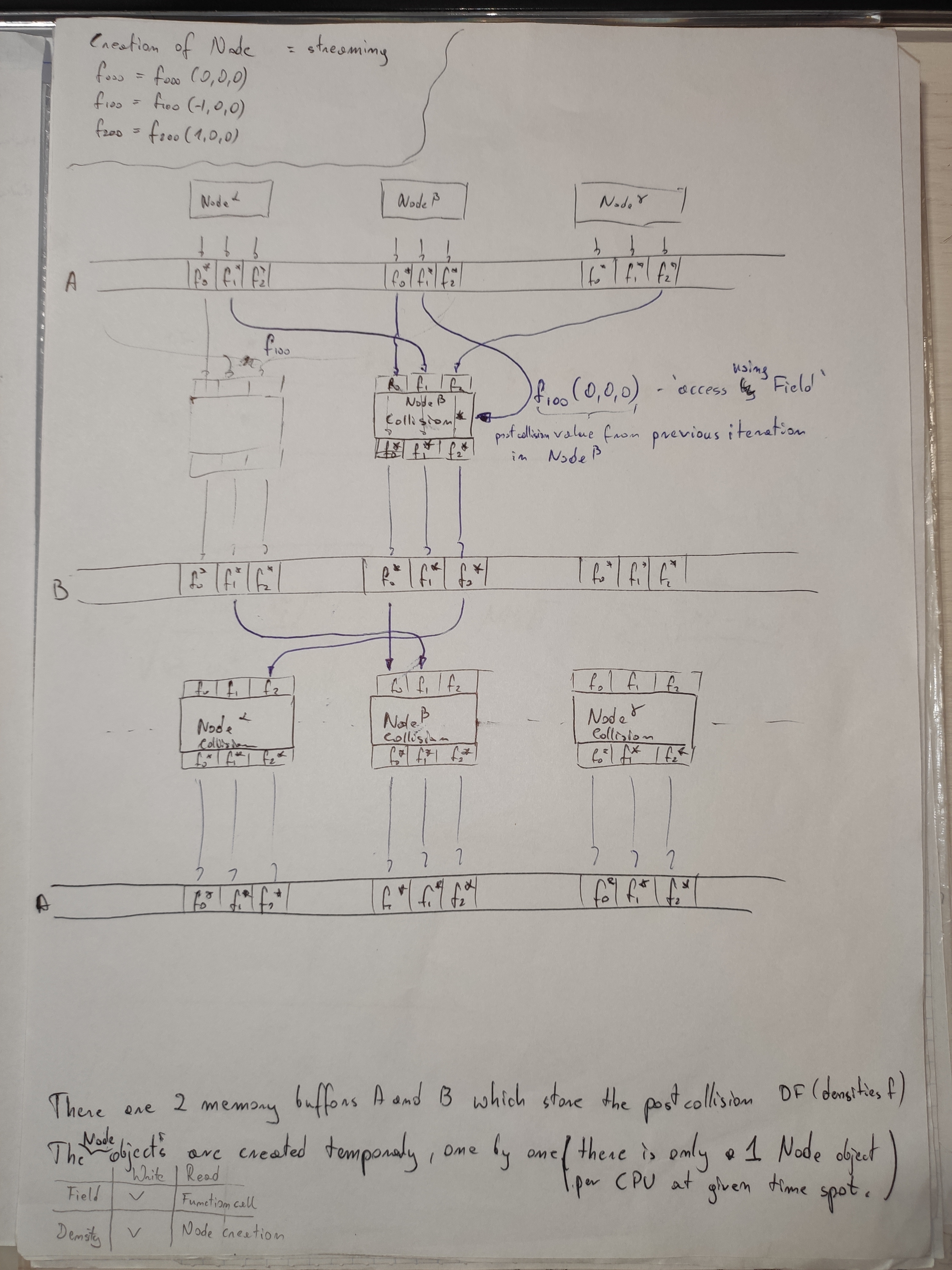
AddField vs AddDensity
| Write | Read | |
|---|---|---|
| Field | x | Function call |
| Density | x | Node Creation (automatically) |
The objects of Node class are created and destroyed 'on the fly' (automatically) during the streaming step.
Notice, that to read the value of the field, it must be called explicitly:
real_t x = myField(0,0) # read myField(0,0)
// do stuff with x
myField = x; // it has to be saved in myField at 0,0 for the next iteration
- AddGlobal - Integrates variables and exports calculated value, useful for calculating forces/fluxes etc.
AddGlobal(name="Name", comment='Some comment', unit="unit")
AddGlobal(name="Flux", comment='Volume flux', unit="m3/s")
- AddSetting - Variables that can be set in the
.xmland accessed byDynamics.cin all nodes. Settings can bezonal, which means that they can be set to different values in different mesh zones, defined in.xmlfiles. It is also possible to define a default value for a setting, this way even if it is not specified in.xmlfile code will run without trouble.
AddSetting(name="Name", default = "value", comment="some comment", zonal=TRUE/FALSE )
AddSetting(name="Velocity", default="0m/s", comment='Inlet velocity', zonal=TRUE)
- AddQuantity - Values that can be exported to VTK files (and Catalyst). In most cases they are macroscopic human-readable quantites like velocity, pressure, displacement etc.
AddQuantity(name="Name", unit="unit", comment="Some comment", vector = T/F)
AddQuantity(name="U", unit="m/s", comment="macroscopic velocity", vector = T)
vector should be set to T for properties like velocity, momentum etc.
In order to extract those values the GetName() function must be defined in Dynamics.c.
- AddNodeType
- BGK
- MRT
- Wall
- Solid
- WVelocity,WPressure,WPressureL
- EVelocity,EPressure,EPressureL
- Inlet
- Outlet
File structure, what are quantities, globals, etc, whats needed in (almost) every model
Stages
Stages are specific functions in Dynamics.c, for which we can define which Densities will be loaded and which Fields will be saved. Stages can be defined in Dynamics.R by:
AddStage("BaseIteration", "Run", save=Fields$group == "f", load=DensityAll$group == "f")
AddStage("CalcRho", save="rho", load=DensityAll$group == "f")
AddStage("CalcNu", save="nu", load=FALSE)
Action is a series of Stages executed in a order. For now there are two meaningful actions:
Iteration, which defines a single (primal) iterationInit, which defines the initialization procedure in each node
Actions can be defined in Dynamics.R by:
AddAction("Iteration", c("BaseIteration","CalcRho","CalcNu"))
Dynamics.C
This file contains the actual 'logic' behind the model. All the calculations are done here. It must contain at least 3 functions to work: Init(), Color(), and Run(). Since CUDA architecture is being used, all the functions need to be preceded by "CudaDeviceFunction".
Init()
Function called to initialise velocity in each node
CudaDeviceFunction void Init() {
// Initialise the velocity at each node
        real_t u[2] = {Velocity, 0.};
        real_t d    = Density;
        SetEquilibrium(d,u);
}
Run()
This function is called each iteration to perform calculations. It should contain instruction for each NodeType used in case. Its general structure looks like this:
CudaDeviceFunction void Run(){
    switch (NodeType & NODE_GROUP){ //Because of the NodeType structure checking must be done this way
                                    // If any SYMMETRY nodes are present, they need to be 'done' first
        case NODE_A:
            A();                    //Function with logic for this NodeType
            break;
        case NODE_B:
            B();
            break;
    }
    switch (NodeType & NODE_GROUP){ //Boundary conditions(BOUNDARY group) must be calculated before collision/streaming
        .
        .
        .
    }
    switch (NodeType & NODE_GROUP){ //Collision/streaming must be done as last step
        .
        .
        .
}
Color()
This function is used to obtain preview during calculations, when not in use it can be only declared without any actual code inside.
CudaDeviceFunction float2 Color() {
        float2 ret;
        vector_t u = getU();
        ret.x = sqrt(u.x*u.x + u.y*u.y);
        if (NodeType == NODE_Solid){
                ret.y = 0;
        } else {
                ret.y = 1;
        }
        return ret;
}
Get()
In order to extract Quantities defined in Dynamics.R we must create function that will compute desired value. Depending on values of vector argument, the Get() function will be either real_t or vector_t type. Below are given examples for the Quantities used most often:
CudaDeviceFunction real_t getRho() {
// This function defines the macroscopic density at the current node.
        return f[8]+f[7]+f[6]+f[5]+f[4]+f[3]+f[2]+f[1]+f[0];
}

CudaDeviceFunction vector_t getU() {
// This function defines the macroscopic velocity at the current node.
        real_t d = f[8]+f[7]+f[6]+f[5]+f[4]+f[3]+f[2]+f[1]+f[0];
        vector_t u;
        // pv = pu + G/2
        u.x = (( f[8]-f[7]-f[6]+f[5]-f[3]+f[1] )/d + GravitationX*0.5 );
        u.y = ((-f[8]-f[7]+f[6]+f[5]-f[4]+f[2] )/d + GravitationY*0.5 );
        u.z = 0;
        return u;
}